Election Predictions’ Dirty Little Secret
When you factor in the errors, they have little predictability
Every presidential election cycle brings intense attention to prediction models like those from FiveThirtyEight and, new this cycle, Nate Silver’s independent model at Silver Bulletin. These models draw from polling data, historical trends (called “fundamentals”), and statistical techniques to forecast outcomes. If you recall feeling let down by FiveThirtyEight’s 71.4% prediction for Hillary Clinton’s 2016 win, you’re not alone; many were surprised when Donald Trump, with a 28.6% chance, emerged as the victor. Theoretically, if we could rerun the 2016 election on 100 identical versions of America with the polling conditions of that year, about 30 of those hypothetical “Americas” would produce a Trump victory. Of course, experimentally preparing 100 “Americas” is impossible, but this thought experiment illustrates the probabilistic nature of election predictions.
Here’s the dirty little secret: the probability of winning is itself an estimate, and it carries its own margin of error. These models report a single percentage for each candidate’s likelihood of winning, yet behind that number lies a broad range of possibilities that vary from simulation to simulation.
Source of Errors: Statistical and Systematic
The well-understood error on any measurement is its statistical error, and pollsters know this. They provide the “margin-of-error” on their poll outcomes, which reflects the statistical error of the sample. The error is inferred from simple counting error, and exists in any measurement that uses discrete counts, as polls do.
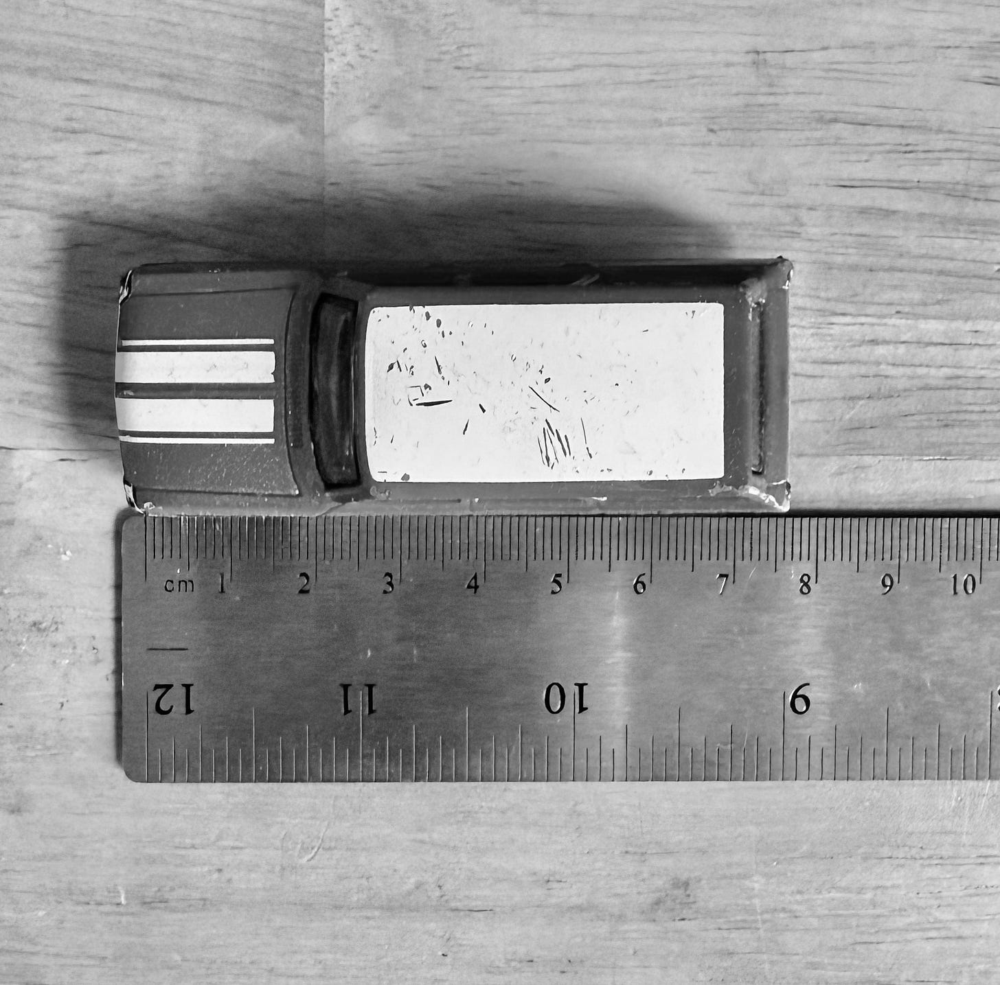
Then, there’s what in physics is called systematic error, meaning that something could be off in your measurement due to the techniques you are using to measure it, like your tool, or that there is an unknown contaminant in the data that skews your error. A simple example of this is measuring something with a ruler. Below, I measured my son’s toy car, and I didn’t properly set the end of the car at the zero of the ruler, so it has what’s called a “zero point” error: I’ve systematically measured it wrong and everything wrong that I would measure in this method, by underestimating its length. I did this by setting the end of the object at the end of the ruler, and not the zero of the measurement marks.

Pollsters are also making this kind of error. It is not intentional, at least, if they’re being proper, unbiased scientists about it. That is, the pollsters effectively don’t know where the “zero point” of their measurement is. They have to estimate it. That is, they have to figure out who is going to vote, and how they are going to vote. As an external observer of the outcomes of the pollsters’ measurements, one gets an estimate of the scale of the systematic error by comparing their results. Note that the pollsters are trying to sample the population in a way that reflects who is going to vote, and how. That includes a model called the voter-turnout model. So, let’s compare two highly-rated pollster’s outcomes for likely voters in Michigan, which is a known critical swing state, from about the same polling time window. Quinnipiac Strategies has Harris up by 4%, and AtlasIntel has Trump up by 3%. That, obviously, is a 7 point difference, which . (They have 538 ratings of 2.8 and 2.7 out of 3, respectively, so very highly rated in methodologies.) One can go through a detailed calculation of t-tests or such to derive the probability of these results actually coming from the same population, but whether it’s 5% or much less than 1% doesn’t matter. They very likely aren’t sampling the same population, and the pollsters will tell you as much: their likely voter models are different. That’s because they all are making at least somewhat if not greatly different models of who will vote.
These different voter models introduce a systematic error, because they make different decisions about who will be voting. How does one take into account systematic error? One method is to average the outcomes of the different pollsters and attribute a new random error associated with how they make their models. This mapping of a systematic offset into a random error relies on the assumption that the likely voter model selection will go to favor one candidate over the other at the same rate as vice-versa. That is, the average of the models’ assumptions is better than any given model. This is likely true in the limit of a large number of models with a wide variety of reasonable choices for models. However, the realm of the unknown unknowns kicks in, where pollsters all make a set of assumptions that give an overwhelming single-sided nature to the systematic errors introduced. After all, both the 2016 and 2020 presidential election polls were overall biased toward the Democratic candidate. There’s discussion that this could be over-corrected in 2024 polls. Overall, the treatment of systematic errors as statistical errors is problematic because these kinds of errors, like the zero point error on the car measurement above, can go more one way than the other. (In more technical terms, systematic errors do not need to follow the central-limit theorem and be normally distributed.)
Nevertheless, the systematic errors are handled as added uncertainty in the prediction platform’s simulations, increasing the overall uncertainty in the election outcome.
The Secret: Overwhelmingly Large Uncertainty in the Outcome
Once the prediction models include an impressive amount of data, their uncertainties, and their covariances (the fact that errors are correlated), they get three numbers: the probability that Harris wins, that Trump wins, or that the electoral college is evenly split at 269-269, leaving the outcome to the House of Representatives. The last case is extremely unlikely in the models, at less than a 1% chance.
There has been much consternation and panic as the predictions over at 538 and Nate Silver’s blog have gotten to favor Trump over Harris at a level of about 53% to 47%. What is hiding in this, in effect, one number of your favored candidate to win is the uncertainties involved. One could ask: how well do we know that Harris is expected to win at 47%, or even more quantitatively, what is the prediction for Harris’ number of the 538 Electoral College votes?
The striking answer is that the uncertainty on the predictions of the Electoral College outcome is enormous. The predictions’ do not provide the standard error (or standard deviation). However, they do provide the range of 95% or 80% of their simulations, for 538, and Nate Silver, respectively. One can then infer the standard error, under the assumption that the distributions are normal (Gaussian). We’re doing this to get at the uncertainty of the prediction. In their most recent forecasts, 538’s standard error for the Electoral College vote is 74, and Silver’s is 46. The fact that Silver’s is smaller is why his has been more sensitive to polling shifts than the 538 model. Things have not changed much in the scale of the uncertainty in the past 8 years. In 2016, the 538 model had a standard error of 57 Electoral College votes.
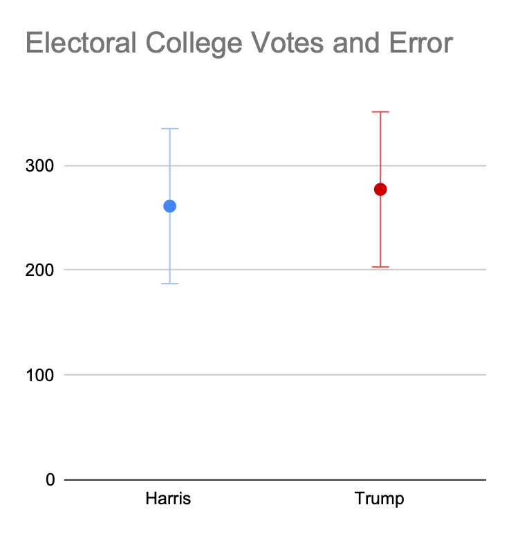
So, to put it in more specific terms, the 538 forecast today for the Electoral College Vote for Harris is 261±74, or a standard error of 28% on the outcome. For Silver, it’s 269±46, or a 17% error. The standard error in a normal distribution only encompasses about two-thirds of outcomes (68.3% to be exact). To put into perspective, this means that there is a one out of three chance that Harris gets either more than 331 Electoral College votes or fewer than 187 Electoral College votes. Or, again, two thirds of the outcomes are that Harris gets between 331 and 187 Electoral College votes, with the remainder of the outcomes outside of that range. Silver’s forecast is a little better in its uncertainty, with a standard-error forecast of between 315 and 223 Electoral College votes.

It goes without saying that a prediction of between 331 and 187 Electoral College votes is not very good, especially when about one third of outcomes will even be outside of this range. See the plot above. If a scientist were to say that there is a significant difference between the measurements of the two points, you would be right to be incredulous.
So, while it is interesting to see how one can try and do a forecast of the outcome, the best models out there are actually not that predictive. And, it’s not like the predictors’ are being dishonest. Both 538 and Silver regularly state that there is a large uncertainty in their predictions, and to not worry about the differences between a 47% win probability and a 53% win probability. However, the scale of the predictions’ uncertainties is truly enormous, and the prediction models’ uncertainties are only shared in one place: their Electoral College vote prediction uncertainties.
All this is to say, in a not so succinct way: the prediction process is interesting and worthy. But, do not worry about the predictions. They have intrinsic limitations. Go out and work to get out the vote, helping your candidate win, and don’t fret about the electoral oracles.
—
Technical note: In talking about the standard deviation of the predictions, I am making the assumption that the distribution is normal or Gaussian. One can see the shape of the 538 and Silver distributions, and they are not Guassian. I’ve adopted that language to more easily give sense of the scale of the uncertainties to those familiar with normal (Gaussian) distributions.


